17. Backpropagation Through Time (part a)
We are now ready to understand how to train the RNN.
When we train RNNs we also use backpropagation, but with a conceptual change. The process is similar to that in the FFNN, with the exception that we need to consider previous time steps, as the system has memory. This process is called Backpropagation Through Time (BPTT) and will be the topic of the next three videos.
- As always, don't forget to take notes.
In the following videos we will use the Loss Function for our error. The Loss Function is the square of the difference between the desired and the calculated outputs. There are variations to the Loss Function, for example, factoring it with a scalar. In the backpropagation example we used a factoring scalar of 1/2 for calculation convenience.
As described previously, the two most commonly used are the Mean Squared Error (MSE) (usually used in regression problems) and the cross entropy (usually used in classification problems).
Here, we are using a variation of the MSE.
19 RNN BPTT A V6 Final
Before diving into Backpropagation Through Time we need a few reminders.
The state vector \bar{s}_t is calculated the following way:
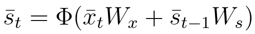
Equation 33
The output vector \bar{y}_t can be product of the state vector \bar{s}_t and the corresponding weight elements of matrix W_y. As mentioned before, if the desired outputs are between 0 and 1, we can also use a softmax function. The following set of equations depicts these calculations:
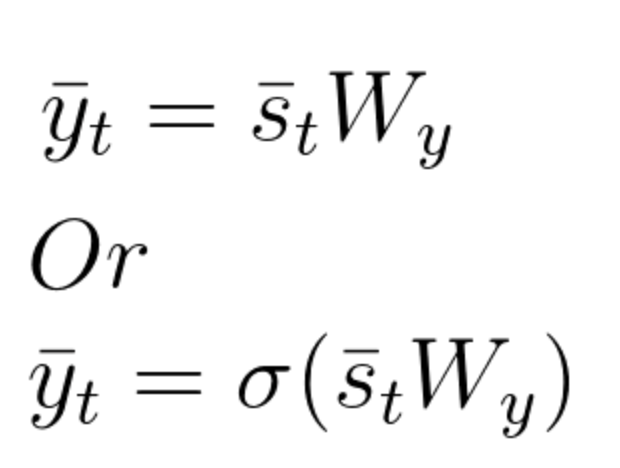
Equation 34
As mentioned before, for the error calculations we will use the Loss Function, where
E_t represents the output error at time t
d_t represents the desired output at time t
y_t represents the calculated output at time t
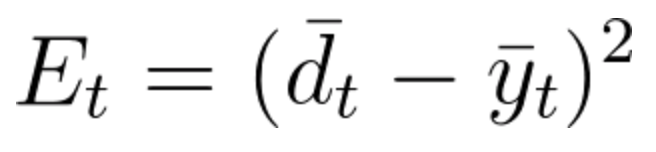
Equation 35
In BPTT we train the network at timestep t as well as take into account all of the previous timesteps.
The easiest way to explain the idea is to simply jump into an example.
In this example we will focus on the BPTT process for time step t=3. You will see that in order to adjust all three weight matrices, W_x, W_s and W_y, we need to consider timestep 3 as well as timestep 2 and timestep 1.
As we are focusing on timestep t=3, the Loss function will be: E_3=(\bar{d}_3-\bar{y}_3)^2
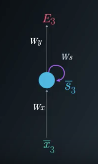
The Folded Model at Timestep 3
To update each weight matrix, we need to find the partial derivatives of the Loss Function at time 3, as a function of all of the weight matrices. We will modify each matrix using gradient descent while considering the previous timesteps.
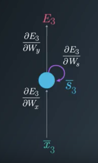
Gradient Considerations in the Folded Model